Inférence pour la tendance a posteriori
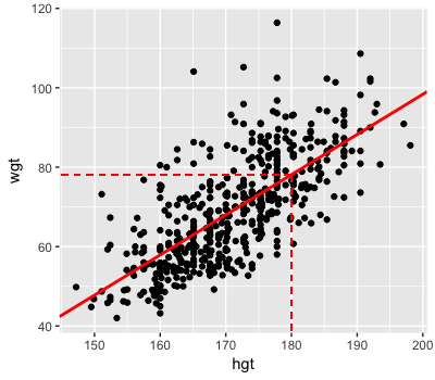
Rappelez-vous la vraisemblance du modèle de régression bayésien du poids \(Y\) par la taille \(X\) : \(Y \sim N(m, s^2)\) où \(m = a + b X\). Dans des exercices précédents, vous avez approximé la forme de la tendance a posteriori \(m\) (ligne pleine). À partir de cela, on remarque que le poids typique pour des adultes mesurant 180 cm est d’environ 80 kg (lignes en pointillé) :
Vous allez utiliser la sortie de simulation RJAGS pour approximer la tendance a posteriori du poids chez les adultes de 180 cm ainsi que l’incertitude a posteriori autour de cette tendance. La simulation RJAGS de 100 000 itérations de l’a posteriori, weight_sim_big, est disponible dans votre espace de travail, ainsi qu’une trame de données contenant la sortie de la chaîne de Markov, weight_chains.
Cet exercice fait partie du cours
<cours>Modélisation bayésienne avec RJAGS</cours>Instructions de l’exercice
weight_chainscontient 100 000 ensembles de valeurs plausibles a posteriori pour les paramètres \(a\) et \(b\). À partir de chacun, calculez le poids moyen (typique) pour des adultes de 180 cm, \(a + b * 180\). Stockez ces tendances dans une nouvelle variablem_180dansweight_chains.Construisez un graphique de densité a posteriori des 100 000 valeurs de
m_180.Utilisez les 100 000 valeurs de
m_180pour calculer un intervalle de crédibilité a posteriori à 95 % pour le poids moyen des adultes mesurant 180 cm.
Exercice interactif pratique
Essayez cet exercice en complétant ce code d’exemple.
# Calculate the trend under each Markov chain parameter set
weight_chains <- weight_chains  %>%
    mutate(m_180 = ___)

# Construct a posterior density plot of the trend
ggplot(___, aes(x = ___)) +
    geom_density()

# Construct a posterior credible interval for the trend
quantile(___, probs = c(___, ___))