后验趋势的推断

回顾按身高 $X$ 拟合体重 $Y$ 的贝叶斯回归模型的似然：$Y \sim N(m, s^2)$，其中 $m = a + b X$。在之前的练习中，您已经近似了后验趋势 $m$ 的形式（实线）。据此可见，身高 180 cm 的成年人，其典型体重大约为 80 kg（虚线）：

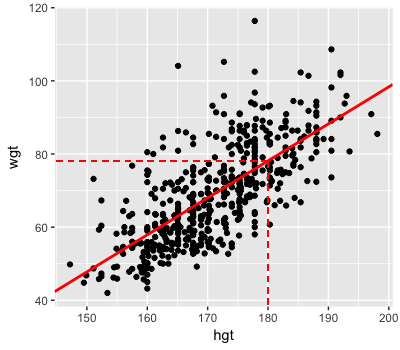
您将使用 RJAGS 的模拟输出来近似身高 180 cm 成年人的体重后验「趋势」，以及该趋势的后验「不确定性」。工作区中提供了对后验进行 100,000 次迭代的 RJAGS 模拟对象 weight_sim_big，以及包含马尔可夫链输出的数据框 weight_chains。

本练习是课程的一部分

使用 RJAGS 的贝叶斯建模

查看课程

练习说明

weight_chains 包含 100,000 组 $a$ 和 $b$ 的后验可信参数取值。对每一组，计算身高 180 cm 成年人的平均（典型）体重，即 $a + b * 180$。将这些趋势保存为 weight_chains 中的新变量 m_180。
绘制 100,000 个 m_180 值的后验密度图。
使用这 100,000 个 m_180 值，计算身高 180 cm 成年人平均体重的 95% 后验置信区间。

交互式实操练习

通过完成这段示例代码来试试这个练习。

# Calculate the trend under each Markov chain parameter set
weight_chains <- weight_chains  %>% 
    mutate(m_180 = ___)

# Construct a posterior density plot of the trend
ggplot(___, aes(x = ___)) + 
    geom_density() 

# Construct a posterior credible interval for the trend
quantile(___, probs = c(___, ___))

编辑并运行代码