La naturaleza recursiva de la varianza GARCH
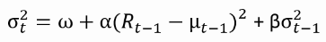
Bajo la ecuación GARCH(1,1), la varianza prevista viene determinada por la sorpresa al cuadrado en el rendimiento y la predicción de varianza anterior:
Puedes implementarlo usando un bucle (consulta las diapositivas si no recuerdas la estructura del bucle del vídeo).
Hagámoslo para los rendimientos diarios del S&P 500. Las variables omega, alpha, beta, nobs, e2 y predvar ya están cargadas en tu entorno de R.
Este ejercicio forma parte del curso
Modelos GARCH en R
Instrucciones del ejercicio
- Calcula las varianzas previstas.
- Usa
predvarpara definir la serie de volatilidad anualizada previstaann_predvol. - Representa la volatilidad anualizada prevista para los años 2008-2009 para ver la dinámica alrededor de la crisis financiera.
ejercicio interactivo práctico
Prueba este ejercicio completando este código de ejemplo.
# Compute the predicted variances
predvar[1] <- var(sp500ret)
for(t in 2:nobs){
   predvar[t] <- ___ + ___ * e2[t-1] + ___ * predvar[___]
}

# Create annualized predicted volatility
ann_predvol <- xts(___(252) * sqrt(___), order.by = time(sp500ret))

# Plot the annual predicted volatility in 2008 and 2009
___(___["2008::2009"], main = "Ann. S&P 500 vol in 2008-2009")