Transformações de entrada: o "hockey stick"

Neste exercício, vamos construir um modelo para prever o preço a partir de uma medida do tamanho da casa (área). O conjunto de dados houseprice, já carregado para você, tem as colunas:

price: preço da casa em unidades de $1000
size: área

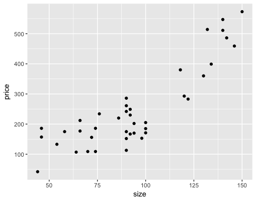
Um diagrama de dispersão mostra que os dados são bastante não lineares: uma espécie de "hockey stick", em que o preço fica relativamente estável para casas menores, mas sobe acentuadamente conforme a casa aumenta. Polinômios de grau 2 (quadráticos) e 3 (cúbicos) costumam ser boas formas funcionais para expressar relações do tipo hockey stick. Observe que pode não haver uma razão "física" para price estar relacionado ao quadrado de size; um quadrático é simplesmente uma aproximação em forma fechada do relacionamento observado.

scatterplot

Você vai ajustar um modelo para prever o preço como função do tamanho ao quadrado e avaliar seu ajuste nos dados de treino.

Como ^ também é um símbolo para expressar interações, use a função I() (docs) para tratar a expressão x^2 “como está”: isto é, como o quadrado de x, e não como a interação de x com ela mesma.

exampleFormula = y ~ I(x^2)

Este exercício faz parte do curso

Aprendizado Supervisionado em R: Regressão

Ver curso

Instruções do exercício

Escreva uma fórmula, fmla_sqr, para expressar price como função de size ao quadrado. Imprima-a.
Ajuste um modelo model_sqr aos dados usando fmla_sqr.
Para comparação, ajuste um modelo linear model_lin aos dados usando a fórmula price ~ size.
Preencha os espaços em branco para
- gerar previsões nos dados de treino a partir dos dois modelos
- pivotar as previsões para uma única coluna pred usando pivot_longer().
- comparar graficamente as previsões dos dois modelos com os dados. Qual se ajusta melhor?

Exercício interativo prático

Experimente este exercício completando este código de exemplo.

# houseprice is available
summary(houseprice)

# Create the formula for price as a function of squared size
(fmla_sqr <- ___)

# Fit a model of price as a function of squared size (use fmla_sqr)
model_sqr <- ___

# Fit a model of price as a linear function of size
model_lin <- ___

# Make predictions and compare
houseprice %>% 
    mutate(pred_lin = ___(___),       # predictions from linear model
           pred_sqr = ___(___)) %>%   # predictions from quadratic model
    pivot_longer(cols = c('pred_lin', 'pred_sqr'), names_to = 'modeltype', values_to = 'pred') %>% # pivot the predictions
    ggplot(aes(x = size)) + 
       geom_point(aes(y = ___)) +                   # actual prices
       geom_line(aes(y = ___, color = modeltype)) + # the predictions
       scale_color_brewer(palette = "Dark2")

Editar e executar o código