输入变换:"冰球杆"
在本练习中,您将基于房屋面积(表面积)来构建一个预测价格的模型。已为您加载的 houseprice 数据集包含以下列:
price:房价,单位为 $1000size:表面积
数据的散点图显示出明显的非线性关系:类似"冰球杆"形状,小户型的价格相对平缓,而随着面积增大,价格急剧上升。二次项和三次项通常是表达这类冰球杆关系的合适函数形式。请注意,price 与 size 的平方之间未必有"物理"上的因果关系;二次式只是对观测到的关系的一种闭式近似。
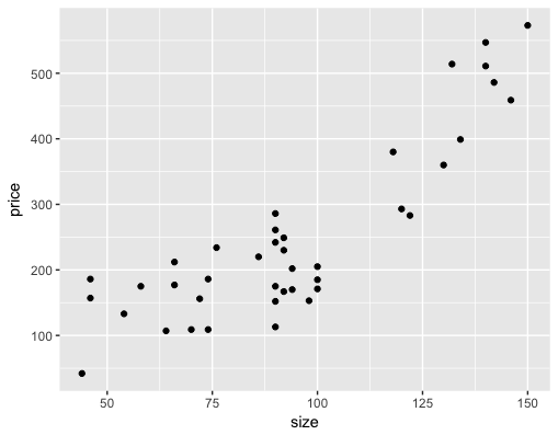
您将拟合一个模型,用面积的平方来预测价格,并查看其在训练数据上的拟合效果。
由于 ^ 也用于表示交互项,请使用函数 I()(文档)将表达式 x^2 按"原样"处理:也就是说,视为 x 的平方,而不是 x 与自身的交互。
exampleFormula = y ~ I(x^2)
本练习是课程的一部分
R 中的监督学习:回归
练习说明
- 编写一个公式
fmla_sqr,将 price 表示为 size 的平方的函数。打印它。 - 使用
fmla_sqr拟合模型model_sqr。 - 作为对比,使用公式
price ~ size拟合线性模型model_lin。 - 填空以:
- 使用这两个模型对训练数据进行预测。
- 使用
pivot_longer()将预测值透视为单列pred。 - 将两个模型的预测与数据进行图形对比。哪个拟合得更好?
交互式实操练习
通过完成这段示例代码来试试这个练习。
# houseprice is available
summary(houseprice)

# Create the formula for price as a function of squared size
(fmla_sqr <- ___)

# Fit a model of price as a function of squared size (use fmla_sqr)
model_sqr <- ___

# Fit a model of price as a linear function of size
model_lin <- ___

# Make predictions and compare
houseprice %>%
    mutate(pred_lin = ___(___),       # predictions from linear model
           pred_sqr = ___(___)) %>%   # predictions from quadratic model
    pivot_longer(cols = c('pred_lin', 'pred_sqr'), names_to = 'modeltype', values_to = 'pred') %>% # pivot the predictions
    ggplot(aes(x = size)) +
       geom_point(aes(y = ___)) +                   # actual prices
       geom_line(aes(y = ___, color = modeltype)) + # the predictions
       scale_color_brewer(palette = "Dark2")