輸入轉換:hockey stick
在這個練習中,你將建立一個模型,根據房屋的大小(面積)來預測價格。已為你載入的 houseprice 資料集包含下列欄位:
price:房價,單位為 $1000size:面積
資料的散佈圖顯示出相當明顯的非線性關係:類似「hockey stick」的形狀——小房子的價格相對平坦,但房屋愈大價格上升愈陡。二次或三次多項式常常能夠良好刻畫這種 hockey stick 式的關係。請注意,price 與 size 的平方之間未必有「物理」上的因果關係;二次式只是對觀察到的關係進行閉形式近似。
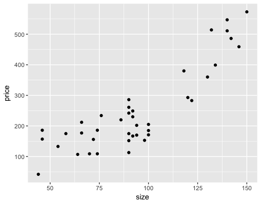
你將擬合一個模型,使用面積的平方來預測價格,並查看其在訓練資料上的擬合情形。
因為 ^ 也可用來表示交互作用,請使用 I() 函式(docs)把運算式 x^2 視為「如其所示」:也就是把它當作 x 的平方,而不是 x 與自身的交互作用。
exampleFormula = y ~ I(x^2)
本練習屬於課程
R 中的監督式學習:回歸
練習說明
- 撰寫一個 formula
fmla_sqr,將 price 表示為 size 的平方函數。並列印它。 - 使用
fmla_sqr對資料擬合模型model_sqr。 - 作為比較,使用公式
price ~ size對資料擬合線性模型model_lin。 - 填空以:
- 從兩個模型針對訓練資料產生預測。
- 使用
pivot_longer()將預測整理為單一欄位pred。 - 以圖形方式將兩個模型的預測與資料相比較。哪一個擬合得更好?
動手互動練習
試著完成這個範例程式碼,體驗一下這個練習。
# houseprice is available
summary(houseprice)

# Create the formula for price as a function of squared size
(fmla_sqr <- ___)

# Fit a model of price as a function of squared size (use fmla_sqr)
model_sqr <- ___

# Fit a model of price as a linear function of size
model_lin <- ___

# Make predictions and compare
houseprice %>%
    mutate(pred_lin = ___(___),       # predictions from linear model
           pred_sqr = ___(___)) %>%   # predictions from quadratic model
    pivot_longer(cols = c('pred_lin', 'pred_sqr'), names_to = 'modeltype', values_to = 'pred') %>% # pivot the predictions
    ggplot(aes(x = size)) +
       geom_point(aes(y = ___)) +                   # actual prices
       geom_line(aes(y = ___, color = modeltype)) + # the predictions
       scale_color_brewer(palette = "Dark2")