dense レイヤー演算を使う
これまでに、線形代数を使って tensorflow で dense レイヤーを定義する方法を見てきました。この演習では、線形代数の詳細は省略し、keras に任せます。これにより、隠れ層が2層・特徴量が10の次のネットワークを、隠れ層1層・特徴量3のネットワークよりも少ないコードで構築できます。
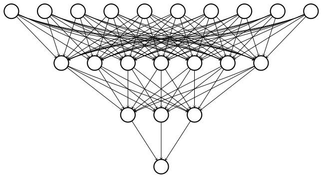
このネットワークを構築するには、3つの dense レイヤーを定義します。各レイヤーは前のレイヤーを入力として受け取り、重みを掛け、活性化関数を適用します。入力データは 100x10 のテンソル borrower_features として定義済みで利用できます。また、keras.layers モジュールも利用可能です。
この演習はコースの一部です
Introduction to TensorFlow in Python
演習の手順
dense1を、出力ノードが7個で活性化関数が sigmoid の dense レイヤーに設定します。dense2を、出力ノードが3個で活性化関数が sigmoid の dense レイヤーとして定義します。predictionsを、出力ノードが1個で活性化関数が sigmoid の dense レイヤーとして定義します。.shapeメソッドを使って、dense1、dense2、predictionsの順に形状を出力してください。これらのテンソルがいずれも100行になるのはなぜでしょうか?
実践的なインタラクティブ演習
このサンプルコードを完成させて、この演習に挑戦してみましょう。
# Define the first dense layer
dense1 = keras.layers.Dense(____, activation='____')(borrower_features)

# Define a dense layer with 3 output nodes
dense2 = ____

# Define a dense layer with 1 output node
predictions = ____

# Print the shapes of dense1, dense2, and predictions
print('\n shape of dense1: ', dense1.shape)
print('\n shape of dense2: ', ____.shape)
print('\n shape of predictions: ', ____.shape)