Transformaciones logarítmicas y de potencia
En el último ejercicio, comparaste las distribuciones de un conjunto de entrenamiento y de prueba de loan_data. Esto es especialmente relevante en una entrevista de Machine Learning, porque la distribución observada determina si necesitas usar técnicas que acerquen la distribución de tus variables a una distribución normal para no violar los supuestos de normalidad.
En este ejercicio, usarás la transformación logarítmica y de potencia del módulo scipy.stats sobre la variable Years of Credit History de loan_data, junto con la función distplot() de seaborn, que representa tanto su distribución como la estimación de densidad por kernel.
Todos los paquetes relevantes ya se han importado por ti.
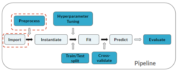
Así es como avanzas en la canalización:
Este ejercicio forma parte del curso
Practicing Machine Learning Interview Questions in Python
ejercicio interactivo práctico
Prueba este ejercicio completando este código de ejemplo.
# Subset loan_data
cr_yrs = ____['____']

# Histogram and kernel density estimate
plt.figure()
sns.____(____)
plt.show()