Logarithmus- und Potenztransformationen
In der letzten Übung hast du die Verteilungen eines Trainings- und Testsets von loan_data verglichen. Das ist in einem Machine-Learning-Interview besonders wichtig, weil die beobachtete Verteilung vorgibt, ob du Techniken einsetzen solltest, die deine Feature-Verteilungen in Richtung Normalverteilung verschieben, damit Normalitätsannahmen nicht verletzt werden.
In dieser Übung verwendest du die Log- und Potenztransformation aus dem Modul scipy.stats auf das Feature Years of Credit History von loan_data zusammen mit der Funktion distplot() aus seaborn, die sowohl die Verteilung als auch die Kernel-Dichteschätzung (KDE) darstellt.
Alle relevanten Pakete wurden bereits für dich importiert.
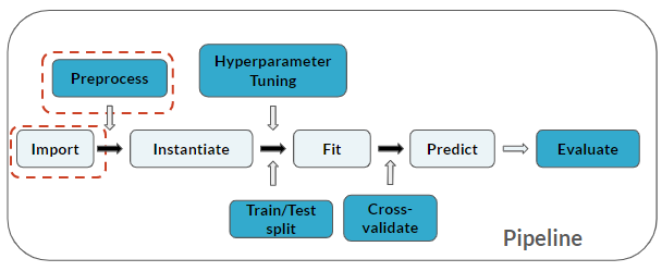
Hier befindest du dich in der Pipeline:
Diese Übung ist Teil des Kurses
<Kurs>ML-Vorstellungsgespräche in Python üben</Kurs>Interaktive praktische Übung
Versuche dich an dieser Übung, indem du diesen Beispielcode vervollständigst.
# Subset loan_data
cr_yrs = ____['____']

# Histogram and kernel density estimate
plt.figure()
sns.____(____)
plt.show()