应用 3：热门婴儿姓名再访

很好！希望您喜欢构建那个用柱形图展示热门婴儿姓名的应用。让我们为本章收个尾，在之前应用的基础上进行增强，添加一个以选项卡形式展示前 10 个婴儿姓名的表格。最终的应用应与下方截图在视觉上相似。

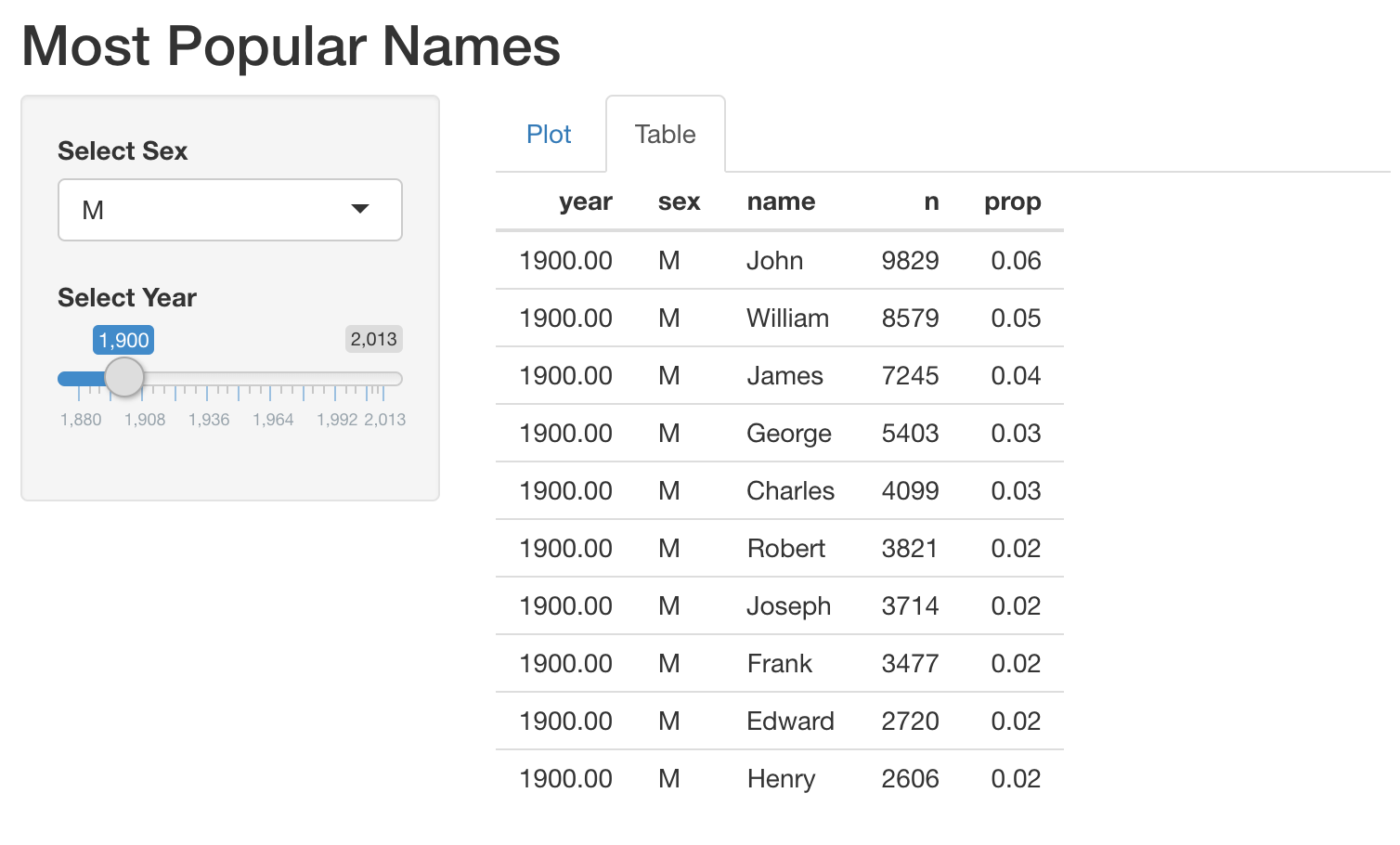
An app where the name selector and year slider appears in the left sidebar, while the graph and table appear as tabs on the right in the main panel

请注意，我们已提供函数 get_top_names()，用于提取给定 year 和 sex 的前 10 个姓名。比如，您可以使用 get_top_names(2000, "M") 获取 2000 年的前 10 个男性姓名。

本练习是课程的一部分

使用 R 构建 Shiny Web 应用

查看课程

练习说明

这里提供的代码来自上一练习中您构建的应用。请修改此代码，在服务器端新增一个输出，用于显示热门姓名的表格。
在 UI 中将图表和表格的输出布局为选项卡（tabs）。

交互式实操练习

通过完成这段示例代码来试试这个练习。

# MODIFY this app (built in the previous exercise)
ui <- fluidPage(
  titlePanel("Most Popular Names"),
  sidebarLayout(
    sidebarPanel(
      selectInput('sex', 'Select Sex', c("M", "F")),
      sliderInput('year', 'Select Year', min = 1880, max = 2017, value = 1900)
    ),
    mainPanel(
     plotOutput('plot')
    )
  )
)

server <- function(input, output, session) {
  output$plot <- renderPlot({
    top_names_by_sex_year <- get_top_names(input$year, input$sex) 
    ggplot(top_names_by_sex_year, aes(x = name, y = prop)) +
      geom_col()
  })
}

shinyApp(ui = ui, server = server)

编辑并运行代码