Transformations logarithmiques et puissances
Dans le dernier exercice, vous avez comparé les distributions d’un jeu d’entraînement et d’un jeu de test de loan_data. C’est un point particulièrement important en entretien Machine Learning, car la distribution observée détermine si vous devez appliquer des techniques qui rapprochent vos variables explicatives d’une distribution normale afin de ne pas violer les hypothèses de normalité.
Dans cet exercice, vous allez utiliser les transformations logarithmique et en puissance du module scipy.stats sur la variable Years of Credit History de loan_data, ainsi que la fonction distplot() de seaborn, qui trace à la fois la distribution et l’estimation de densité par noyau.
Tous les packages pertinents ont été importés pour vous.
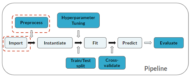
Voici où vous en êtes dans le pipeline :
Cet exercice fait partie du cours
<cours>S’entraîner aux questions d’entretien en Machine Learning avec Python</cours>Exercice interactif pratique
Essayez cet exercice en complétant ce code d’exemple.
# Subset loan_data
cr_yrs = ____['____']

# Histogram and kernel density estimate
plt.figure()
sns.____(____)
plt.show()