Variation in Two Parts

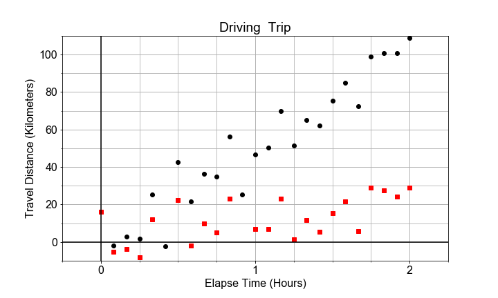
Given two data sets of distance-versus-time data, one with very small velocity and one with large velocity. Notice that both may have the same standard error of slope, but different R-squared for the model overall, depending on the size of the slope ("effect size") as compared to the standard error ("uncertainty").

If we plot both data sets as scatter plots on the same axes, the contrast is clear. Variation due to the slope is different than variation due to the random scatter about the trend line. In this exercise, your goal is to compute the standard error and R-squared for two data sets and compare.

This exercise is part of the course

Introduction to Linear Modeling in Python

View Course

Exercise instructions

Build and fit() an ols() model, for both data sets distances1 and distances2.
Use the .bse of resulting models model_1 and model_2, and the 'times' key to extract the standard error values for the slope from each model.
Use the .rsquared attribute to extract the R-squared value from each model.
Print the resulting se_1, rsquared_1, se_2, rsquared_2, and visually compare.

Hands-on interactive exercise

Have a go at this exercise by completing this sample code.

# Build and fit two models, for columns distances1 and distances2 in df
model_1 = ols(formula="____ ~ times", data=df).____()
model_2 = ols(formula="____ ~ times", data=df).____()

# Extract R-squared for each model, and the standard error for each slope
se_1 = model_1.____['times']
se_2 = model_2.____['times']
rsquared_1 = model_1.____
rsquared_2 = model_2.____

# Print the results
print('Model 1: SE = {:0.3f}, R-squared = {:0.3f}'.format(____, ____))
print('Model 2: SE = {:0.3f}, R-squared = {:0.3f}'.format(____, ____))

Edit and Run Code