Log and power transformations

In the last exercise, you compared the distributions of a training set and test set of loan_data. This is especially poignant in a machine learning interview because the distribution observed dictates whether or not you need to use techniques which nudge your feature distributions toward a normal distribution so that normality assumptions are not violated.

In this exercise, you will be using the log and power transformation from the scipy.stats module on the Years of Credit History feature of loan_data along with the distplot() function from seaborn, which plots both its distribution and kernel density estimation.

All relevant packages have been imported for you.

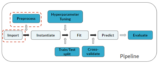
Here is where you are in the pipeline:

Machine learning pipeline

Bu egzersiz

Practicing Machine Learning Interview Questions in Python

kursunun bir parçasıdır

Kursu Görüntüle

Uygulamalı interaktif egzersiz

Bu örnek kodu tamamlayarak bu egzersizi bitirin.

# Subset loan_data
cr_yrs = ____['____']

# Histogram and kernel density estimate
plt.figure()
sns.____(____)
plt.show()

Kodu Düzenle ve Çalıştır