L’algèbre linéaire des couches denses

Il existe deux façons de définir une couche dense dans tensorflow. La première s’appuie sur des opérations d’algèbre linéaire de bas niveau. La seconde utilise des opérations de haut niveau via keras. Dans cet exercice, nous allons utiliser la première méthode pour construire le réseau illustré dans l’image ci-dessous.

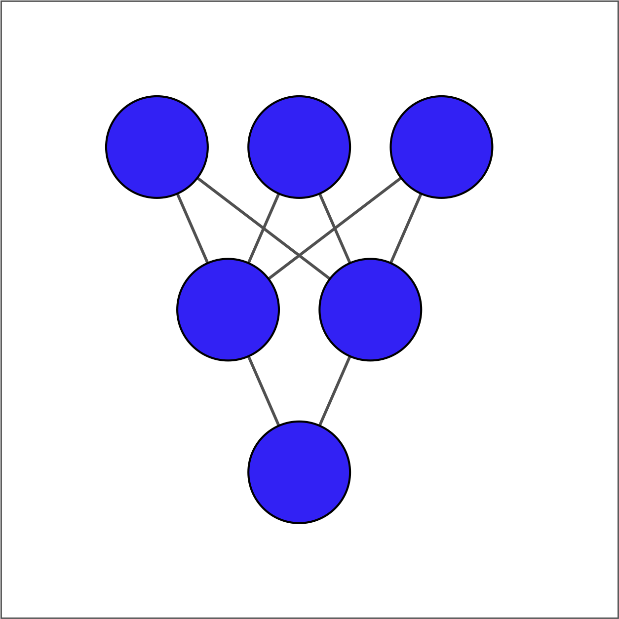
Cette image représente un réseau de neurones avec 5 nœuds d’entrée et 3 nœuds de sortie.

La couche d’entrée contient 3 variables — niveau d’études, situation matrimoniale et âge — disponibles sous le nom borrower_features. La couche cachée contient 2 nœuds et la couche de sortie contient un seul nœud.

Pour chaque couche, vous prendrez la couche précédente en entrée, initialiserez un jeu de poids, calculerez le produit des entrées par les poids, puis appliquerez une fonction d’activation. Notez que Variable(), ones(), matmul() et keras() ont été importés depuis tensorflow.

Cet exercice fait partie du cours

Introduction à TensorFlow en Python

Afficher le cours

Exercice interactif pratique

Essayez cet exercice en complétant cet exemple de code.

# Initialize bias1
bias1 = Variable(1.0)

# Initialize weights1 as 3x2 variable of ones
weights1 = ____(ones((____, ____)))

# Perform matrix multiplication of borrower_features and weights1
product1 = ____

# Apply sigmoid activation function to product1 + bias1
dense1 = keras.activations.____(____ + ____)

# Print shape of dense1
print("\n dense1's output shape: {}".format(dense1.shape))

Modifier et exécuter le code

Cet exercice fait partie du cours

Introduction à TensorFlow en Python

IntermédiaireNiveau de compétence

4.8+

Commencer le cours gratuitement

Avant de pouvoir construire des modèles avancés dans TensorFlow 2, vous devez d’abord en maîtriser les bases. Dans ce chapitre, vous apprendrez à définir des constantes et des variables, à effectuer des additions et multiplications de tenseurs, et à calculer des dérivées. Des notions d’algèbre linéaire seront utiles, mais ne sont pas indispensables.

Exercise 1: Constantes et variables Exercise 2: Définir des données comme constantes Exercise 3: Définir des variables Exercise 4: Opérations de base Exercise 5: Réaliser une multiplication élément par élément Exercise 6: Réaliser des prédictions avec une multiplication de matrices Exercise 7: Sommer sur les dimensions d’un tenseur Exercise 8: Opérations avancées Exercise 9: Remodeler des tenseurs Exercise 10: Optimiser avec les gradients Exercise 11: Travailler avec des données d’images

Dans ce chapitre, vous apprendrez à construire, résoudre et utiliser des modèles dans TensorFlow 2 pour faire des prédictions. Vous vous concentrerez sur une classe de modèles simple — la régression linéaire — et tenterez de prédire les prix de l’immobilier. À la fin du chapitre, vous saurez charger et manipuler des données, construire des fonctions de perte, effectuer une minimisation, faire des prédictions et réduire l’utilisation des ressources avec l’entraînement par lots.

Exercise 1: Données d’entrée Exercise 2: Charger des données avec pandas Exercise 3: Définir le type de données Exercise 4: Fonctions de perte Exercise 5: Fonctions de perte dans TensorFlow Exercise 6: Modifier la fonction de perte Exercise 7: Régression linéaire Exercise 8: Mettre en place une régression linéaire Exercise 9: Entraîner un modèle linéaire Exercise 10: Régression linéaire multiple Exercise 11: Entraînement par lots Exercise 12: Préparer l’entraînement par lots Exercise 13: Entraîner un modèle linéaire par lots

Les chapitres précédents vous ont appris à construire des modèles dans TensorFlow 2. Dans ce chapitre, vous appliquerez ces mêmes outils pour construire, entraîner et utiliser des réseaux de neurones pour faire des prédictions. Vous apprendrez à définir des couches denses, à appliquer des fonctions d’activation, à choisir un optimiseur et à utiliser la régularisation pour réduire le surapprentissage. Vous profiterez de la flexibilité de TensorFlow en combinant l’algèbre linéaire de bas niveau et les opérations de l’API Keras de haut niveau pour définir et entraîner des modèles.

Exercise 1: Couches denses Exercise 2: L’algèbre linéaire des couches denses

Exercice en cours

Exercise 3: L’approche bas niveau avec plusieurs exemples Exercise 4: Utiliser l’opération de couche dense Exercise 5: Fonctions d’activation Exercise 6: Problèmes de classification binaire Exercise 7: Problèmes de classification multiclasse Exercise 8: Optimiseurs Exercise 9: Les dangers des minima locaux Exercise 10: Éviter les minima locaux Exercise 11: Entraîner un réseau dans TensorFlow Exercise 12: Initialisation dans TensorFlow Exercise 13: Définir le modèle et la fonction de perte Exercise 14: Entraîner des réseaux de neurones avec TensorFlow

Dans le chapitre final, vous utiliserez des API de haut niveau de TensorFlow 2 pour entraîner un classificateur de lettres en langue des signes. Vous utiliserez les API Keras séquentielle et fonctionnelle pour entraîner, valider, faire des prédictions avec et évaluer des modèles. Vous apprendrez également à utiliser l’API Estimators pour simplifier la définition et l’entraînement des modèles et réduire les risques d’erreurs.

Exercise 1: Définir des réseaux de neurones avec Keras Exercise 2: Le modèle séquentiel avec Keras Exercise 3: Compiler un modèle séquentiel Exercise 4: Définir un modèle à entrées multiples Exercise 5: Entraînement et validation avec Keras Exercise 6: Entraîner avec Keras Exercise 7: Métriques et validation avec Keras Exercise 8: Détection du surapprentissage Exercise 9: Évaluer des modèles Exercise 10: Entraîner des modèles avec l’API Estimators Exercise 11: Préparer l’entraînement avec les Estimators Exercise 12: Définir des Estimators Exercise 13: Félicitations !