Visually Estimating the Slope & Intercept
Building linear models is an automated way of doing something we can roughly do "manually" with data visualization and a lot of trial-and-error. The visual method is not the most efficient or precise method, but it does illustrate the concepts very well, so let's try it!
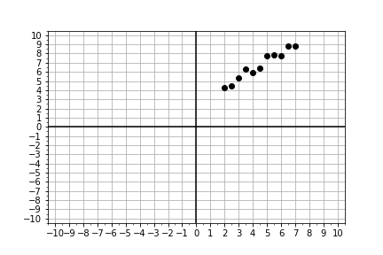
Given some measured data, your goal is to guess values for slope and intercept, pass them into the model, and adjust your guess until the resulting model fits the data. Use the provided data xd, yd, and the provided function model() to create model predictions. Compare the predictions and data using the provided plot_data_and_model().
This exercise is part of the course
Introduction to Linear Modeling in Python
Exercise instructions
- Inspect the chart above, and provide preliminary estimates of
trial_slopeandtrial_intercept. These can be adjusted later in the exercise. - Use the predefined function
xm, ym = model(intercept, slope)to generate model predictions. - Use the provided function
fig = plot_data_and_model(xd, yd, xm, ym)to plot the measured data(xd, yd)and the modeled predictions(xm, ym)together. - If the model does not fit the data, try different values for
trial_slopeandtrial_interceptand rerun your code. - Repeat until you believe you have the best values, and then assign them to
final_slopeandfinal_interceptand submit your answer.
Hands-on interactive exercise
Have a go at this exercise by completing this sample code.
# Look at the plot data and guess initial trial values
trial_slope = ____
trial_intercept = ____

# input thoses guesses into the model function to compute the model values.
xm, ym = ____(trial_intercept, trial_slope)

# Compare your your model to the data with the plot function
fig = ____(xd, yd, xm, ym)
plt.show()

# Repeat the steps above until your slope and intercept guess makes the model line up with the data.
final_slope = ____
final_intercept = ____