Seizoens-ACF en -PACF
Hieronder zie je een tijdreeks met het geschatte aantal waterverbruikers in Londen. Met het blote oog zie je geen duidelijke seizoenspatronen, maar je ogen zijn niet je beste hulpmiddel.
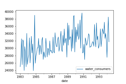
In deze oefening gebruik je de ACF en PACF om deze data op seizoensinvloeden te testen. Je ziet in de bovenstaande grafiek dat de tijdreeks niet stationair is, dus je kunt hem beter detrenden. Je doet dit door het voortschrijdend gemiddelde af te trekken. Onthoud dat je een venstergrootte kunt kiezen die groter is dan de waarschijnlijke periode.
De functie plot_acf() is geïmporteerd en de tijdreeks is ingeladen als water.
Deze oefening maakt deel uit van de cursus
ARIMA-modellen in Python
Interactieve oefening met praktijkervaring
Probeer deze oefening door deze voorbeeldcode aan te vullen.
# Create figure and subplot
fig, ax1 = plt.subplots()

# Plot the ACF on ax1
plot_acf(____, ____, zero=False,  ax=ax1)

# Show figure
plt.show()