글머리 기호 목록 만들기
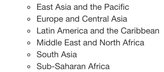
이전에, 대상 독자에게 추가 정보를 제공하기 위해 Markdown 파일에 텍스트를 추가하는 방법을 배웠어요. 이제 investment_annual_summary 데이터에 포함된 지역을 명시하는 글머리 기호 목록을 만들어 볼게요. 아래 비디오의 이미지를 참고해, 표에 포함해야 할 지역 목록을 다시 떠올려 보세요.
이 연습은 강의의 일부입니다
R Markdown으로 보고서 만들기
연습 안내
- 보고서의
27번 줄부터, 데이터에 포함된 각 지역의 글머리 기호 목록을 추가하세요: East Asia and the Pacific, Europe and Central Asia, Latin America and the Caribbean, Middle East and North Africa, South Asia, 그리고 Sub-Saharan Africa.
실습형 인터랙티브 연습
이 예제를 이 샘플 코드를 완성하여 풀어보세요.
{"investment_report.Rmd":"---\ntitle: \"Investment Report\"\ndate: \"`r format(Sys.time(), '%d %B %Y')`\"\noutput: html_document\n---\n\n```{r setup, include = FALSE}\nknitr::opts_chunk$set(fig.align = 'center', echo = TRUE)\n```\n\n```{r data, include = FALSE}\nlibrary(readr)\nlibrary(dplyr)\nlibrary(ggplot2)\n\ninvestment_annual_summary <- read_csv(\"https://assets.datacamp.com/production/repositories/5756/datasets/d0251f26117bbcf0ea96ac276555b9003f4f7372/investment_annual_summary.csv\")\ninvestment_region_summary <- read_csv(\"https://assets.datacamp.com/production/repositories/5756/datasets/52f5414f6504e0503e86eb1043afa9b3d157fab2/investment_region_summary.csv\")\ninvestment_services_projects <- read_csv(\"https://assets.datacamp.com/production/repositories/5756/datasets/bcb2e39ecbe521f4b414a21e35f7b8b5c50aec64/investment_services_projects.csv\")\n```\n\n\n## Datasets \n### Investment Annual Summary\nThe `investment_annual_summary` dataset provides a summary of the dollars in millions provided to each of the following regions for each fiscal year, from 2012 to 2018:\n\n\n\n\n\n\n\n\n```{r investment-annual-summary, out.width = '85%', fig.cap = 'Figure 1.1 The Investment Annual Summary for each region for 2012 to 2018.'}\nggplot(investment_annual_summary, aes(x = fiscal_year, y = dollars_in_millions, color = region)) +\n geom_line() +\n labs(\n title = \"Investment Annual Summary\",\n x = \"Fiscal Year\",\n y = \"Dollars in Millions\"\n )\n```\n\n### Investment Projects in Brazil\nThe `investment_services_projects` dataset provides information about each investment project from 2012 to 2018. Information listed includes the project name, company name, sector, project status, and investment amounts.\n\n```{r brazil-investment-projects, out.width = '95%', fig.cap = 'Figure 1.2 The Investment Services Projects in Brazil from 2012 to 2018.'}\nbrazil_investment_projects <- investment_services_projects %>%\n filter(country == \"Brazil\") \n\nggplot(brazil_investment_projects, aes(x = date_disclosed, y = total_investment, color = status)) +\n geom_point() +\n labs(\n title = \"Investment Services Projects in Brazil\",\n x = \"Date Disclosed\",\n y = \"Total IFC Investment in Dollars in Millions\"\n )\n```\n\n### Investment Projects in Brazil in 2018\nThe `investment_services_projects` dataset was filtered below to focus on information about each investment project from the 2018 fiscal year, and is referred to as `brazil_investment_projects_2018`. \n\n```{r brazil-investment-projects-2018, out.width = '95%', fig.cap = 'Figure 1.3 The Investment Services Projects in Brazil in 2018.'}\nbrazil_investment_projects_2018 <- investment_services_projects %>%\n filter(country == \"Brazil\",\n date_disclosed >= \"2017-07-01\",\n date_disclosed <= \"2018-06-30\") \n\nggplot(brazil_investment_projects_2018, aes(x = date_disclosed, y = total_investment, color = status)) +\n geom_point() +\n labs(\n title = \"Investment Services Projects in Brazil in 2018\",\n x = \"Date Disclosed\",\n y = \"Total IFC Investment in Dollars in Millions\"\n ) \n```\n\n\n"}