App 3: Beliebte Babynamen – Redux
Super! Hoffentlich hat dir die App gefallen, die beliebte Babynamen als Säulendiagramm zeigt. Lass uns dieses Kapitel abschließen, indem wir die App von vorhin erweitern und einen Tab mit einer Tabelle der Top 10 Babynamen hinzufügen. Deine finale App sollte dem Screenshot unten optisch ähneln.
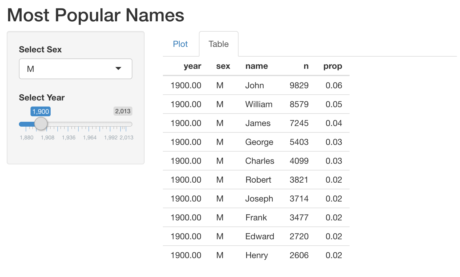
Beachte, dass wir eine Funktion get_top_names() bereitgestellt haben, um die Top 10 Namen für ein bestimmtes year und sex zu ermitteln. Du kannst die Top 10 männlichen Namen für das Jahr 2000 mit get_top_names(2000, "M") abrufen.
Diese Übung ist Teil des Kurses
<Kurs>Webanwendungen mit Shiny in R entwickeln</Kurs>Übungsanweisungen
- Der bereitgestellte Code stammt aus der App, die du in der vorherigen Übung gebaut hast. Ändere den Code so, dass im Server eine Ausgabe hinzugefügt wird, die eine Tabelle mit beliebten Namen anzeigt.
- Lege die Plot- und Tabellen-Ausgaben im UI als Tabs an.
Interaktive praktische Übung
Versuche dich an dieser Übung, indem du diesen Beispielcode vervollständigst.
# MODIFY this app (built in the previous exercise)
ui <- fluidPage(
  titlePanel("Most Popular Names"),
  sidebarLayout(
    sidebarPanel(
      selectInput('sex', 'Select Sex', c("M", "F")),
      sliderInput('year', 'Select Year', min = 1880, max = 2017, value = 1900)
    ),
    mainPanel(
     plotOutput('plot')
    )
  )
)

server <- function(input, output, session) {
  output$plot <- renderPlot({
    top_names_by_sex_year <- get_top_names(input$year, input$sex)
    ggplot(top_names_by_sex_year, aes(x = name, y = prop)) +
      geom_col()
  })
}

shinyApp(ui = ui, server = server)