Seasonal ACF and PACF
Below is a time series showing the estimated number of water consumers in London. By eye you can't see any obvious seasonal pattern, however your eyes aren't the best tools you have.
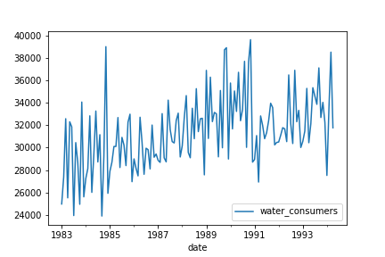
In this exercise you will use the ACF and PACF to test this data for seasonality. You can see from the plot above that the time series isn't stationary, so you should probably detrend it. You will detrend it by subtracting the moving average. Remember that you could use a window size of any value bigger than the likely period.
The plot_acf() function has been imported and the time series has been loaded in as water.
Este ejercicio forma parte del curso
ARIMA Models in Python
ejercicio interactivo práctico
Prueba este ejercicio completando este código de ejemplo.
# Create figure and subplot
fig, ax1 = plt.subplots()

# Plot the ACF on ax1
plot_acf(____, ____, zero=False,  ax=ax1)

# Show figure
plt.show()