Inference for the posterior trend

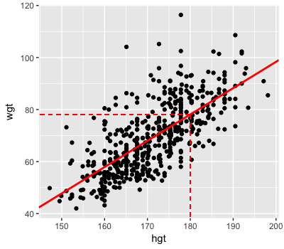
Recall the likelihood of the Bayesian regression model of weight \(Y\) by height \(X\): \(Y \sim N(m, s^2)\) where \(m = a + b X\). In earlier exercises you approximated the form of the posterior trend \(m\) (solid line). From this, notice that the typical weight among 180 cm adults is roughly 80 kg (dashed lines):

You will use RJAGS simulation output to approximate the posterior trend in weight among 180 cm tall adults as well as the posterior uncertainty in this trend. The 100,000 iteration RJAGS simulation of the posterior, weight_sim_big, is in your workspace along with a data frame of the Markov chain output, weight_chains.

This exercise is part of the course

Bayesian Modeling with RJAGS

View Course

Exercise instructions

weight_chains contains 100,000 sets of posterior plausible parameter values of \(a\) and \(b\). From each, calculate the mean (typical) weight among 180 cm tall adults, \(a + b * 180\). Store these trends as a new variable m_180 in weight_chains.
Construct a posterior density plot of 100,000 m_180 values.
Use the 100,000 m_180 values to calculate a 95% posterior credible interval for the mean weight among 180 cm tall adults.

Hands-on interactive exercise

Have a go at this exercise by completing this sample code.

# Calculate the trend under each Markov chain parameter set
weight_chains <- weight_chains  %>% 
    mutate(m_180 = ___)

# Construct a posterior density plot of the trend
ggplot(___, aes(x = ___)) + 
    geom_density() 

# Construct a posterior credible interval for the trend
quantile(___, probs = c(___, ___))

Edit and Run Code