ACF et PACF saisonniers

Ci-dessous se trouve une série temporelle représentant l’estimation du nombre de consommateurs d’eau à Londres. À l’œil nu, vous ne distinguez pas de saisonnalité évidente, mais vos yeux ne sont pas vos meilleurs outils.

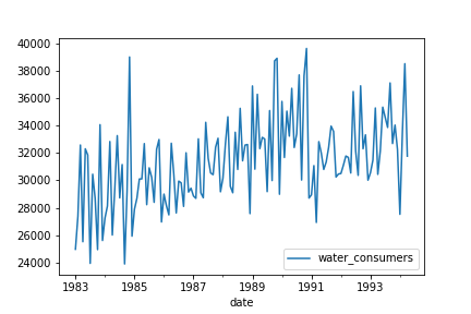
Dans cet exercice, vous allez utiliser l’ACF et la PACF pour tester la saisonnalité de ces données. Le graphique ci-dessus montre que la série n’est pas stationnaire ; vous devriez donc probablement la détrendiser. Vous allez le faire en soustrayant la moyenne mobile. Rappelez-vous que vous pouvez choisir une fenêtre de n’importe quelle taille supérieure à la période probable.

La fonction plot_acf() a été importée et la série temporelle a été chargée sous le nom water.

Cet exercice fait partie du cours

Modèles ARIMA en Python

Afficher le cours

Exercice interactif pratique

Essayez cet exercice en complétant cet exemple de code.

# Create figure and subplot
fig, ax1 = plt.subplots()

# Plot the ACF on ax1
plot_acf(____, ____, zero=False,  ax=ax1)

# Show figure
plt.show()

Modifier et exécuter le code

Cet exercice fait partie du cours

Modèles ARIMA en Python

AvancéNiveau de compétence

4.9+

Commencer le cours gratuitement

Plongez directement au cœur du sujet et découvrez les propriétés essentielles des séries temporelles. Vous verrez ce qu’est la stationnarité et pourquoi elle est importante pour les modèles ARMA. Vous apprendrez à tester la stationnarité à l’œil et avec un test statistique standard. Enfin, vous étudierez la structure de base des modèles ARMA, générerez des données ARMA et ajusterez un modèle ARMA.

Exercise 1: Introduction aux séries temporelles et à la stationnarité Exercise 2: Exploration Exercise 3: Découper en ensembles d’entraînement et de test Exercise 4: Est-elle stationnaire Exercise 5: Rendre les séries temporelles stationnaires Exercise 6: Dickey-Fuller augmenté Exercise 7: Prendre la différence Exercise 8: Autres transformations Exercise 9: Introduction aux modèles AR, MA et ARMA Exercise 10: Ordre du modèle Exercise 11: Générer des données ARMA Exercise 12: Préambule à l’ajustement

Dans ce chapitre, c’est à vous de prévoir ce qui attend vos données. Vous apprendrez à utiliser l’élégant package statsmodels pour ajuster des modèles ARMA, ARIMA et ARMAX. Ensuite, vous utiliserez vos modèles pour prédire l’avenir incertain des cours boursiers !

Exercise 1: Ajuster des modèles de séries temporelles Exercise 2: Ajuster des modèles AR et MA Exercise 3: Ajuster un modèle ARMA Exercise 4: Ajuster un modèle ARMAX Exercise 5: Prévisions Exercise 6: Générer des prévisions à un pas Exercise 7: Tracer des prévisions à un pas d’avance Exercise 8: Générer des prévisions dynamiques Exercise 9: Tracer des prévisions dynamiques Exercise 10: Introduction aux modèles ARIMA Exercise 11: Différenciation et ajustement d’un ARMA Exercise 12: Dérouler une prévision ARMA Exercise 13: Ajuster un modèle ARIMA Exercise 14: Choisir un modèle ARIMA

Dans ce chapitre, vous deviendrez un modélisateur au jugement affûté. Vous apprendrez à identifier des ordres de modèles prometteurs à partir des données elles-mêmes, puis, une fois les meilleurs modèles entraînés, vous verrez comment choisir le modèle optimal parmi cette sélection ajustée. Vous découvrirez aussi un excellent cadre pour structurer vos projets de séries temporelles.

Exercise 1: Introduction à l’ACF et à la PACF Exercise 2: AR ou MA Exercise 3: Ordre des tremblements de terre Exercise 4: Introduction à l’AIC et au BIC Exercise 5: Recherche de l’ordre du modèle Exercise 6: Choisir l’ordre avec l’AIC et le BIC Exercise 7: AIC et BIC vs ACF et PACF Exercise 8: Diagnostic du modèle Exercise 9: Erreur absolue moyenne Exercise 10: Statistiques récapitulatives de diagnostic Exercise 11: Tracer les diagnostics Exercise 12: Méthode de Box-Jenkins Exercise 13: Identification Exercise 14: Identification II Exercise 15: Estimation Exercise 16: Diagnostics

Dans ce dernier chapitre, vous apprendrez à utiliser des modèles ARIMA saisonniers pour ajuster des données plus complexes. Vous verrez comment décomposer ces données en composantes saisonnières et non saisonnières, puis vous aurez l’occasion de mobiliser tous vos outils ARIMA dans un ultime défi de prévision à l’échelle mondiale.

Exercise 1: Séries temporelles saisonnières Exercise 2: Décomposition saisonnière Exercise 3: ACF et PACF saisonniers

Exercice en cours

Exercise 4: Modèles SARIMA Exercise 5: Ajuster des modèles SARIMA Exercise 6: Choisir l’ordre SARIMA Exercise 7: Prévisions SARIMA vs ARIMA Exercise 8: Automatisation et sauvegarde Exercise 9: Sélection automatisée de modèles Exercise 10: Enregistrer et mettre à jour des modèles Exercise 11: SARIMA et Box-Jenkins Exercise 12: Saisonnalité multiplicative vs additive Exercise 13: Diagnostic du modèle SARIMA Exercise 14: Prévision SARIMA Exercise 15: Félicitations !