Input transforms: the "hockey stick"
In this exercise, we will build a model to predict price from
a measure of the house's size (surface area). The houseprice dataset, loaded for you, has the columns:
price: house price in units of $1000size: surface area
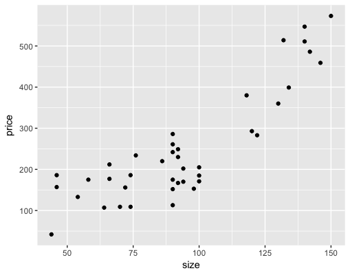
A scatterplot of the data shows that the data is quite non-linear: a sort of "hockey-stick" where price is fairly flat for smaller houses, but rises steeply as the house gets larger. Quadratics and tritics are often good functional forms to express hockey-stick like relationships. Note that there may not be a "physical" reason that price is related to the square of the size; a quadratic is simply a closed form approximation of the observed relationship.
You will fit a model to predict price as a function of the squared size, and look at its fit on the training data.
Because ^ is also a symbol to express interactions, use the function I() (docs) to treat the expression x^2 “as is”: that is, as the square of x rather than the interaction of x with itself.
exampleFormula = y ~ I(x^2)
This exercise is part of the course
Supervised Learning in R: Regression
Exercise instructions
- Write a formula,
fmla_sqr, to express price as a function of squared size. Print it. - Fit a model
model_sqrto the data usingfmla_sqr - For comparison, fit a linear model
model_linto the data using the formulaprice ~ size. - Fill in the blanks to
- make predictions from the training data from the two models
- pivot the predictions into a single column
predusingpivot_longer(). - graphically compare the predictions of the two models to the data. Which fits better?
Hands-on interactive exercise
Have a go at this exercise by completing this sample code.
# houseprice is available
summary(houseprice)

# Create the formula for price as a function of squared size
(fmla_sqr <- ___)

# Fit a model of price as a function of squared size (use fmla_sqr)
model_sqr <- ___

# Fit a model of price as a linear function of size
model_lin <- ___

# Make predictions and compare
houseprice %>%
    mutate(pred_lin = ___(___),       # predictions from linear model
           pred_sqr = ___(___)) %>%   # predictions from quadratic model
    pivot_longer(cols = c('pred_lin', 'pred_sqr'), names_to = 'modeltype', values_to = 'pred') %>% # pivot the predictions
    ggplot(aes(x = size)) +
       geom_point(aes(y = ___)) +                   # actual prices
       geom_line(aes(y = ___, color = modeltype)) + # the predictions
       scale_color_brewer(palette = "Dark2")