The linear algebra of dense layers

There are two ways to define a dense layer in tensorflow. The first involves the use of low-level, linear algebraic operations. The second makes use of high-level keras operations. In this exercise, we will use the first method to construct the network shown in the image below.

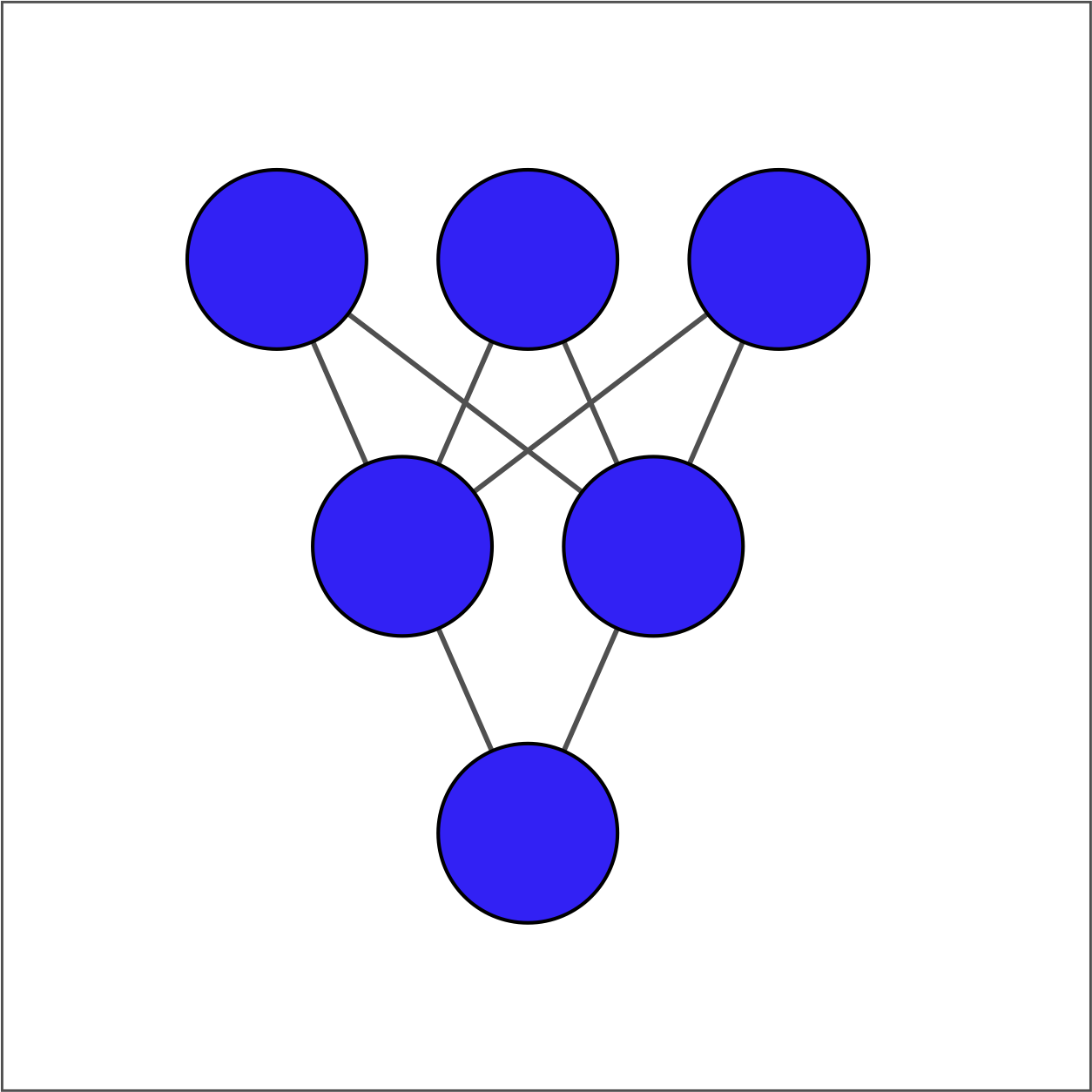
This image depicts an neural network with 5 input nodes and 3 output nodes.

The input layer contains 3 features -- education, marital status, and age -- which are available as borrower_features. The hidden layer contains 2 nodes and the output layer contains a single node.

For each layer, you will take the previous layer as an input, initialize a set of weights, compute the product of the inputs and weights, and then apply an activation function. Note that Variable(), ones(), matmul(), and keras() have been imported from tensorflow.

This exercise is part of the course

Introduction to TensorFlow in Python

Hands-on interactive exercise

Have a go at this exercise by completing this sample code.

# Initialize bias1
bias1 = Variable(1.0)

# Initialize weights1 as 3x2 variable of ones
weights1 = ____(ones((____, ____)))

# Perform matrix multiplication of borrower_features and weights1
product1 = ____

# Apply sigmoid activation function to product1 + bias1
dense1 = keras.activations.____(____ + ____)

# Print shape of dense1
print("\n dense1's output shape: {}".format(dense1.shape))

Edit and Run Code

This exercise is part of the course

Introduction to TensorFlow in Python

IntermediateSkill Level

4.8+

Start Course for Free

Before you can build advanced models in TensorFlow 2, you will first need to understand the basics. In this chapter, you’ll learn how to define constants and variables, perform tensor addition and multiplication, and compute derivatives. Knowledge of linear algebra will be helpful, but not necessary.

Exercise 1: Constants and variables Exercise 2: Defining data as constants Exercise 3: Defining variables Exercise 4: Basic operations Exercise 5: Performing element-wise multiplication Exercise 6: Making predictions with matrix multiplication Exercise 7: Summing over tensor dimensions Exercise 8: Advanced operations Exercise 9: Reshaping tensors Exercise 10: Optimizing with gradients Exercise 11: Working with image data

In this chapter, you will learn how to build, solve, and make predictions with models in TensorFlow 2. You will focus on a simple class of models – the linear regression model – and will try to predict housing prices. By the end of the chapter, you will know how to load and manipulate data, construct loss functions, perform minimization, make predictions, and reduce resource use with batch training.

Exercise 1: Input data Exercise 2: Load data using pandas Exercise 3: Setting the data type Exercise 4: Loss functions Exercise 5: Loss functions in TensorFlow Exercise 6: Modifying the loss function Exercise 7: Linear regression Exercise 8: Set up a linear regression Exercise 9: Train a linear model Exercise 10: Multiple linear regression Exercise 11: Batch training Exercise 12: Preparing to batch train Exercise 13: Training a linear model in batches

The previous chapters taught you how to build models in TensorFlow 2. In this chapter, you will apply those same tools to build, train, and make predictions with neural networks. You will learn how to define dense layers, apply activation functions, select an optimizer, and apply regularization to reduce overfitting. You will take advantage of TensorFlow's flexibility by using both low-level linear algebra and high-level Keras API operations to define and train models.

Exercise 1: Dense layers Exercise 2: The linear algebra of dense layers

Current Exercise

Exercise 3: The low-level approach with multiple examples Exercise 4: Using the dense layer operation Exercise 5: Activation functions Exercise 6: Binary classification problems Exercise 7: Multiclass classification problems Exercise 8: Optimizers Exercise 9: The dangers of local minima Exercise 10: Avoiding local minima Exercise 11: Training a network in TensorFlow Exercise 12: Initialization in TensorFlow Exercise 13: Defining the model and loss function Exercise 14: Training neural networks with TensorFlow

In the final chapter, you'll use high-level APIs in TensorFlow 2 to train a sign language letter classifier. You will use both the sequential and functional Keras APIs to train, validate, make predictions with, and evaluate models. You will also learn how to use the Estimators API to streamline the model definition and training process, and to avoid errors.

Exercise 1: Defining neural networks with Keras Exercise 2: The sequential model in Keras Exercise 3: Compiling a sequential model Exercise 4: Defining a multiple input model Exercise 5: Training and validation with Keras Exercise 6: Training with Keras Exercise 7: Metrics and validation with Keras Exercise 8: Overfitting detection Exercise 9: Evaluating models Exercise 10: Training models with the Estimators API Exercise 11: Preparing to train with Estimators Exercise 12: Defining Estimators Exercise 13: Congratulations!