Exercise

The recursive nature of the GARCH variance

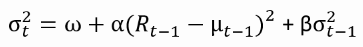
Under the GARCH(1,1) equation the predicted variance is determined by the squared surprise in return and the previous variance prediction:

You can implement this using a loop (refer to the slides if you don't remember the loop structure from the video).

Let's do this for the S&P 500 daily returns. The variables omega, alpha, beta, nobs, e2 and predvar are already loaded in your R environment.

Instructions

100 XP

Compute the predicted variances.
Use predvar to define the series of predicted annualized volatility ann_predvol .
Plot the predicted annualized volatility for the years 2008-2009 to see the dynamics around the financial crisis.