Monte Carlo sampling for discrete-event models

Imagine a factory that produces wall clocks. The clocks have been growing in popularity, and now the demand is higher than the production capacity. The factory has been working at full capacity for months, and you want to understand its behavior and bottlenecks better so that more informed management decisions can be made and plan future investments and expansion.

A discrete-event model of the factory processes has been developed, and now you want to run a Monte Carlo sampling analysis to explore scenarios. The manufacturing process is summarized in the table below, and the information has been stored in a list of dictionaries named processes, with one dictionary per process. The keys of this dictionary correspond to the table column headers. The following packages have been imported for you: numpy as np, matplotlib.pyplot as plt, seaborn as sns, random, pandas as pd, and time.

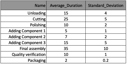
Table with process names and their duration statistics, namely mean and standard deviation.

The Monte-Carlo sampling loop will produce a series of possible process trajectories, as shown in the figure. Monte Carlo trajectories for different process scenario.

This exercise is part of the course

Discrete Event Simulation in Python

View Course

Exercise instructions

Set up the main Monte Carlo sampling for-loop for n_trajectories samples with dummy variable t.
Use the Gaussian distribution from the random package to pseudo-randomly estimate the process duration.

Hands-on interactive exercise

Have a go at this exercise by completing this sample code.

n_trajectories = 100

# Run a Monte-Carlo for-loop for n_trajectories samples
____

    for p in range(len(processes)):
        proc_p = processes[p]

        # Random gauss method to pseudo-randomly estimate process duration
        process_duration = ____(proc_p["Average_Duration"], proc_p["Standard_Deviation"])
        time_record[p + 1] = time_record[p] + process_duration

    df_disc = pd.DataFrame({cNam[0]: process_line_space, cNam[1]: time_record})
    fig = sns.lineplot(data=df_disc, x=cNam[0], y=cNam[1], marker="o")  # Step_10
    fig.set(xlim=(0, len(processes) + 1))
    plt.plot()
plt.grid()
plt.show()

Edit and Run Code