Gradient boosted portfolio performance

At this point you've looked at predicting probability of default using both a LogisticRegression() and XGBClassifier(). You've looked at some scoring and have seen samples of the predictions, but what is the overall affect on portfolio performance? Try using expected loss as a scenario to express the importance of testing different models.

A data frame called portfolio has been created to combine the probabilities of default for both models, the loss given default (assume 20% for now), and the loan_amnt which will be assumed to be the exposure at default.

The data frame cr_loan_prep along with the X_train and y_train training sets have been loaded into the workspace.

This exercise is part of the course

Credit Risk Modeling in Python

View Course

Exercise instructions

Print the first five rows of portfolio.
Create the expected_loss column for the gbt and lr model named gbt_expected_loss and lr_expected_loss.
Print the sum of lr_expected_loss for the entire portfolio.
Print the sum of gbt_expected_loss for the entire portfolio.

Hands-on interactive exercise

Have a go at this exercise by completing this sample code.

# Print the first five rows of the portfolio data frame
print(____.____())

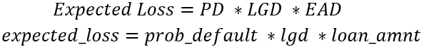
# Create expected loss columns for each model using the formula
portfolio[____] = portfolio[____] * portfolio[____] * portfolio[____]
portfolio[____] = portfolio[____] * portfolio[____] * portfolio[____]

# Print the sum of the expected loss for lr
print('LR expected loss: ', np.____(____[____]))

# Print the sum of the expected loss for gbt
print('GBT expected loss: ', np.____(____[____]))

Edit and Run Code