App 3: Popular Baby Names Redux
Great! Hope you enjoyed building that app displaying popular baby names as a column plot. Let us wrap this chapter up by enhancing the app we built earlier by adding a table showing the top 10 baby names as a tab. Your final app should visually resemble the screenshot below.
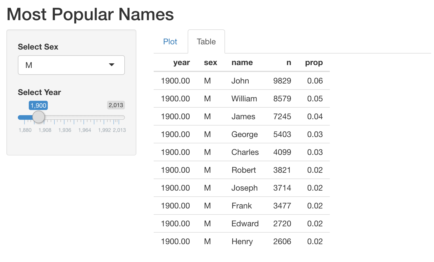
Note that we have provided a function get_top_names() to extract
the top 10 names for a given year and sex. You can get the top 10 male names
for the year 2000 using get_top_names(2000, "M").
This exercise is part of the course
Building Web Applications with Shiny in R
Exercise instructions
- The code provided is for the app you built in the previous exercise. Modify this code to add an output to the server to display a table of popular names.
- Lay out the plot and table outputs in the UI as tabs.
Hands-on interactive exercise
Have a go at this exercise by completing this sample code.
# MODIFY this app (built in the previous exercise)
ui <- fluidPage(
  titlePanel("Most Popular Names"),
  sidebarLayout(
    sidebarPanel(
      selectInput('sex', 'Select Sex', c("M", "F")),
      sliderInput('year', 'Select Year', min = 1880, max = 2017, value = 1900)
    ),
    mainPanel(
     plotOutput('plot')
    )
  )
)

server <- function(input, output, session) {
  output$plot <- renderPlot({
    top_names_by_sex_year <- get_top_names(input$year, input$sex)
    ggplot(top_names_by_sex_year, aes(x = name, y = prop)) +
      geom_col()
  })
}

shinyApp(ui = ui, server = server)